PVsyst 3D Near Shading Scene Builder — Ground-Mount Modeling Tutorial

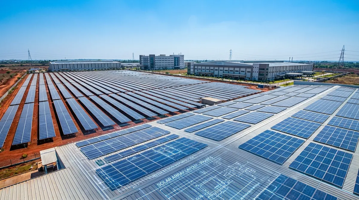
The PVsyst 3D near shading scene builder is where inter-row shading, terrain effects, and near-horizon obstructions get translated into the loss fractions that appear in your bankable energy yield report. For a utility-scale ground-mount project — a 10 MW tracker array in Rajasthan or a 5 MW fixed-tilt ground-mount in North Carolina — the 3D scene is the geometric foundation that determines how accurately PVsyst models the optical shading loss between rows, the bifacial rear irradiance, and the string-level partial shading effects.

Most engineers running PVsyst for the first time treat the 3D near shading module as an optional step — entering a shading factor manually instead of building the scene. This produces a faster workflow but a less defensible simulation. Independent engineers reviewing bankable IEAs for IREDA, IFC, or US tax equity expect the simulation to include a geometry-derived near shading calculation, not a manually entered guess. The 3D scene is not optional for a well-documented utility-scale report.

Direct answer. The PVsyst 3D near shading scene builder (accessible from the Project → Near Shadings menu) allows you to define the exact array geometry — row tilt, pitch, row height, number of rows, table width — and then calculate the optical near shading loss as a function of sun position throughout the year. For a properly modeled ground-mount with standard GCR (Ground Coverage Ratio), near shading loss typically ranges from 1.5–4.0%. The scene also drives bifacial rear irradiance calculation if bifacial mode is enabled. Building an accurate 3D scene takes 4–12 hours for a standard utility-scale project; the result is a defensible, geometry-derived shading loss table that replaces manual loss estimates in the simulation.

---

Why the 3D Scene Matters in a Bankable Yield Report

The near shading loss is the energy lost because one row of modules blocks sunlight from reaching the row behind it during morning and evening hours — and during winter months when the sun tracks lower across the sky. For a fixed-tilt system at 22° tilt in India with a pitch-to-height ratio of 3.0, this optical inter-row shading might contribute 1.5–2.5% to annual energy loss. For a tightly packed system at GCR 0.45, it might reach 3.5–5.0%.

The difference between a manually estimated 2.0% and a geometry-derived 3.5% near shading loss is a yield difference of 1.5% — which for a 50 MW project at ₹3.50/kWh PPA represents approximately ₹90–100 lakh in annual revenue. At 25 years, that is a ₹22–25 crore discrepancy in lifetime revenue projections.

---

Step-by-Step: Building the 3D Scene for a Ground-Mount Project

The PVsyst 3D Near Shading module is accessed from the main simulation project via Project → Near Shadings → Edit/Display 3D Scene. The workflow has five stages.

Stage 1 — Project Geometry Parameters

Before opening the 3D scene, confirm the following project parameters that feed into the scene:

1. Site location and orientation — latitude, longitude, and the plane orientation (tilt and azimuth) must be set in the main project before building the 3D scene. The scene inherits these values.

2. Module dimensions — the physical dimensions of the selected module (width, length in meters) must be confirmed from the module datasheet. PVsyst uses these to define the table dimensions.

3. Table layout — the number of modules per string in portrait orientation (typically 1 module per landscape row × N modules in portrait string), and the number of strings per inverter.

For a standard 1P (one module in portrait, landscape rows) fixed-tilt configuration with 550 Wp bifacial modules:

• Module dimensions: approximately 2.279 m × 1.134 m (commercial bifacial 550W)
• Table configuration: 2 modules stacked in portrait = 2.268 m table height
• String: 20–28 modules per string depending on inverter Vmp range

---

Key Parameters: Tilt, Pitch, and the Shading Optimization

The relationship between tilt, pitch, and inter-row shading is the central design optimization problem for fixed-tilt ground-mount projects. PVsyst’s 3D scene is the best tool for quantifying this relationship.

Shading vs Pitch — Typical Relationship for India (Latitude 20°N, 550W Bifacial, 2P Portrait Stack):

Pitch (m)	GCR	Near Shading Loss (%)	Annual Yield (MWh/MWp)	Land Area per MWp (acres)
4.0	0.56	5.5–7.0	1,580–1,620	2.5–2.8
5.0	0.45	2.8–4.0	1,630–1,660	3.0–3.3
6.0	0.37	1.5–2.5	1,650–1,680	3.6–3.9
7.0	0.32	0.8–1.5	1,655–1,685	4.2–4.5
8.0	0.28	0.4–0.9	1,657–1,687	4.8–5.2

The table shows that yield improvement from increasing pitch above 6.0 m is relatively small (1–3 MWh/MWp/year) while land area requirement increases substantially. For projects where land cost is significant (leased land above ₹1 lakh/acre/year), the optimal pitch is typically 5.5–6.5 m. For projects on low-cost owned land, 7.0–8.0 m may be the financial optimum despite the higher land area.

---

Ground-Mount Tilt Angle Selection Using PVsyst

Tilt angle affects both annual yield and inter-row shading. The interaction is significant: a higher tilt angle captures more winter irradiance (where the sun is lower) but also creates a taller shadow that requires greater row pitch for the same shading loss.

Optimal Tilt by Latitude (Fixed-Tilt, South-Facing):

Site Latitude	Rule-of-Thumb Optimal Tilt	PVsyst Recommended Range	Notes
10°N (Tamil Nadu coast)	10–13°	10–15°	Low seasonal variation; flat tilt also practical
15°N (Karnataka, AP)	14–18°	13–20°	Moderate winter benefit from steeper tilt
20°N (Rajasthan, Gujarat)	18–22°	17–24°	Balance of annual yield and winter production
25°N (Punjab, Haryana)	22–26°	20–28°	Greater winter enhancement from steeper tilt
30°N (Himachal, J&K)	26–32°	25–35°	Steep tilt for winter sun; also snow-shedding
35°N (US Southwest)	30–35°	28–38°	Latitude-1° rule applies
40°N (US Northeast)	35–40°	33–42°	Winter production significant for annual optimization

The PVsyst parametric tilt optimization is accessed via Design → System → Tilt optimization. Running 5–8 tilt values from 10–35° produces an annual yield curve. The optimal tilt is where the curve peaks — typically within 2–4° of local latitude for fixed-tilt systems in moderate climates.

Interaction Between Tilt and Pitch:

For a given GCR, higher tilt angles produce more shading. The “no-shading at winter solstice noon” criterion is a useful heuristic: pitch = row_height_at_top × 1/tan(90 − latitude − 23.5°) × sun-factor.

For a 22° tilt system in Rajasthan (latitude 26°N):

• Row height at top: 2.27 m (2P table) × sin(22°) = 0.85 m above bottom-module edge
• Shadow length at winter solstice noon: 0.85 / tan(90 − 26 − 23.5) = 0.85 / tan(40.5°) ≈ 1.0 m
• Minimum pitch to avoid winter solstice noon shading: module_width × cos(22°) + shadow_length ≈ 2.27 × 0.93 + 1.0 ≈ 3.1 m

In practice, most designers target a pitch of 5.5–6.5 m for 22° tilt at 26°N latitude — accepting some early-morning and late-afternoon shading in winter months while minimizing land use.

---

Terrain Modeling — Sloped and Irregular Ground

For sites with significant terrain slope, the PVsyst 3D scene needs to account for the varying row heights that result from ground slope. A slope of 5% means a 5 m rise over 100 m horizontal distance — significant enough to affect inter-row shading when south-facing arrays are laid on north-to-south slopes.

Terrain Impact on Shading:

Terrain Type	Effect on Near Shading	PVsyst Handling
Flat (< 1% slope)	Minimal; standard pitch calculation applies	No terrain adjustment needed
Gentle slope (1–5%)	Moderate; downhill rows shade uphill rows more	Use terrain slope input in 3D scene
Moderate slope (5–10%)	Significant; pitch may need to be increased on downhill grades	Full terrain DXF import or manual slope entry
Steep slope (> 10%)	Major impact; row layout may need to follow contours	Full terrain model; east-west tracking may be preferable
Complex terrain	Site-specific; cross-valley shading may dominate	DXF terrain import with survey data

Importing Terrain from DXF:

For large utility-scale projects on sloped terrain, PVsyst accepts DXF terrain files. The workflow:

1. Obtain a surveyed terrain model as a DXF file (from GPS survey or drone photogrammetry)
2. In the 3D scene: File → Import Terrain → select the DXF file
3. PVsyst renders the terrain as a 3D surface
4. Place the PV plane objects on the terrain surface; PVsyst adjusts row heights automatically
5. Run the near shading calculation with terrain-aware geometry

---

Single-Axis Tracker Shading in PVsyst

Single-axis tracker systems (SAT) add complexity to the 3D shading scene because the row tilt angle changes continuously throughout the day as the tracker follows the sun. PVsyst models SAT shading with a dedicated tracker simulation mode.

Tracker Configuration in PVsyst:

In the 3D scene, select Object Type → Single-Axis Tracker. Configure:

• Axis orientation — horizontal N-S axis is standard for most utility-scale ground-mount
• Maximum tilt angle — typically ±55–60° from horizontal
• Backtracking algorithm — whether the tracker uses backtracking to avoid inter-row shading at low sun angles

Backtracking — Why It Matters:

Without backtracking, early-morning and late-afternoon inter-row shading on tracker systems can be 3–5% of annual yield. With backtracking, the tracker tilts toward horizontal at low sun angles to prevent the shadow from Row N falling on Row N+1, at the cost of not tracking the sun optimally.

PVsyst models both strategies:

• No backtracking: Higher shading loss but better tracking at all times when not shaded
• Ideal backtracking: Eliminates inter-row beam shading; tracker accepts slight non-optimal orientation
• Custom algorithm: For manufacturers with proprietary algorithms different from the ideal backtracking formula

For most utility-scale SAT projects, ideal backtracking reduces near shading loss from 3–5% (no backtracking) to 0.5–1.5%, with a net yield benefit of 1.5–3.5%. The PVsyst Tracker Yield Study Methodology post covers the full tracker optimization workflow in detail.

Tracker Configuration	Near Shading Loss	Typical Annual Yield (MWh/MWp, India 20°N)	Land Requirement
Fixed tilt 20°, pitch 6m	1.5–2.5%	1,640–1,680	3.6–3.9 acres/MWp
SAT, no backtracking, GCR 0.4	3.0–5.0%	1,700–1,740	3.5–3.8 acres/MWp
SAT, backtracking, GCR 0.4	0.5–1.5%	1,750–1,800	3.5–3.8 acres/MWp
SAT, backtracking, GCR 0.35	0.3–0.8%	1,760–1,810	4.0–4.3 acres/MWp

---

Bifacial Module 3D Scene Setup

For bifacial modules, the 3D scene does more than calculate front-side shading — it also calculates the rear irradiance contribution from ground-reflected irradiance, sky diffuse, and beam reflections.

Bifacial Parameters in PVsyst 3D Scene:

To enable bifacial simulation:

1. In the system definition, select a bifacial module (.pan file with bifaciality factor)
2. In Near Shadings settings, enable “Bifacial simulation”
3. Set the ground albedo value (fraction of ground reflectance)
4. Set the row height (distance from ground to lowest module edge)
5. Set the ground clearance

Ground Albedo Values:

Ground Surface	Albedo Range	Notes
Bare soil (typical)	0.15–0.25	Most common for ground-mount; seasonal variation
Dry sand / desert	0.25–0.35	Higher albedo; favorable for bifacial in Rajasthan
Gravel / white gravel	0.25–0.40	White gravel increasing albedo is a documented yield improvement strategy
Green vegetation	0.18–0.25	Agrivoltaic sites; variable by crop type and season
Concrete or white membrane	0.35–0.50	Flat-roof BIPV or white-membrane rooftop systems
Snow (fresh)	0.70–0.90	Temporary high-albedo event; usually averaged over year
Standard assumption (no data)	0.20	PVsyst default; acceptable for initial simulation

Bifacial Gain — Typical Values by Configuration:

Row Height (m)	Ground Albedo	Pitch (m)	Bifacial Gain (%)
0.3 (low clearance)	0.20	6.0	2.5–3.5
0.8 (standard)	0.20	6.0	3.5–5.0
1.5 (high clearance, tracker)	0.20	6.5	4.5–6.5
1.5 (high clearance, tracker)	0.30	6.5	6.0–8.0
1.5 (high clearance, tracker)	0.20	5.0	3.5–5.0 (more inter-row shading reduces rear)

The PVsyst bifacial gain modeling guide covers the bifacial calculation methodology in detail, including the view factor model and how module frameless vs framed construction affects the calculation.

---

Common 3D Scene Errors and Fixes

#	Error	Symptom	Fix
1	Module dimensions entered incorrectly (wrong model)	Shading result doesn’t match physical layout	Verify module .pan file dimensions match the selected module; re-enter manually if needed
2	Pitch entered as module-edge-to-module-edge instead of center-to-center	GCR calculated incorrectly; scene looks compressed	Re-enter pitch as center-to-center (horizontal) distance between row centerlines
3	Tilt angle inconsistent between system definition and 3D scene	Shading factors don’t apply correctly to simulation	Ensure tilt in 3D scene matches the system plane orientation
4	No backtracking selected for SAT system	Near shading loss unrealistically high (3–5% instead of 0.5–1.5%)	Enable ideal backtracking in tracker configuration
5	Bifacial mode not enabled despite bifacial module selection	Bifacial gain = 0% in output; simulation underestimates yield	Enable bifacial in Near Shadings settings; set ground albedo
6	Ground albedo set to 0.50 without justification	Over-estimates bifacial gain; IE will flag	Use 0.20 default unless site has documented higher albedo; cite source
7	3D scene not applied to simulation (still using manual shading fraction)	Simulation ignores 3D scene results	In Near Shadings: set to “According to module layout (Shading Fraction)“
8	Terrain assumed flat when site has > 5% slope	Under-estimates shading on downhill rows	Import terrain DXF or set terrain slope in 3D scene

---

Validation — Comparing 3D Scene Output Against Rules of Thumb

After building the 3D scene and running the near shading calculation, validate the output against the following rules of thumb before proceeding to the full simulation:

1. Near shading loss within expected range — For a standard fixed-tilt ground-mount at GCR 0.38–0.45, near shading should be 1.5–3.5%. If the result is outside this range, review pitch, tilt, and row height inputs.

2. Bifacial gain in expected range — For an open-rack tracker system at 1.5 m height with albedo 0.20, bifacial gain should be 4–7%. Outside this range suggests incorrect height, albedo, or scene geometry.

3. PR in expected range post-shading — After including near shading in the full simulation, check PR. For an Indian ground-mount with typical losses, PR 0.76–0.82 is expected. Significantly outside this range warrants a full loss input review.

4. Shading loss lower for SAT with backtracking than fixed tilt — SAT with backtracking at comparable GCR should produce near shading 0.5–1.5% vs 1.5–3.0% for fixed tilt. If SAT shading is higher than fixed tilt, backtracking may not be enabled.

---

Exporting and Documenting the 3D Scene for IEA Reports

The bankable IEA report must include documentation of the 3D scene geometry to allow IE review and reproduction. Standard documentation package:

1. 3D scene screenshots — top view, south-facing isometric view, and a close-up showing row geometry with dimensions labeled
2. Key geometric parameters table — tilt, pitch, row height, ground clearance, table width, number of rows, GCR, azimuth
3. Near shading loss value — annual percentage and the shading factor table as a CSV export
4. Bifacial parameters — if applicable: ground albedo, row height, bifaciality factor, bifacial gain result
5. Terrain description — flat or sloped; if sloped, the slope gradient and terrain model source

This documentation set is typically presented as Section 3 of the PVsyst simulation report (after Section 1 site data and Section 2 system definition). IEs reviewing IREDA or IFC-financed projects will confirm that the 3D scene geometry matches the as-designed layout.

---

How Heaven Designs Builds 3D Scenes for Utility-Scale Projects

Heaven Designs delivers PVsyst 3D scene builds as part of the ground-mount design package, with the near shading computation, bifacial configuration, and scene documentation included in every bankable yield report.

• Solar Ground Mount Design — Utility-scale PVsyst simulation with full 3D scene build, SAT backtracking analysis, bifacial optimization, and IREDA-format IEA report.
• Solar Rooftop Detailed Engineering Design — Commercial and utility-scale rooftop PVsyst with 3D obstruction modeling and bifacial gain analysis.
• Solar 3D Pre-Design — Rapid 48-hour pre-design with Helioscope 3D scene for sales-stage layout before PVsyst commitment.
• Site Survey and Land Feasibility — Drone survey and terrain model as PVsyst terrain input for complex terrain sites.

Related posts: PVsyst Loss Diagram Interpretation | PVsyst Bifacial Gain Modeling Tutorial | PVsyst Tracker Yield Study Methodology | PVsyst vs Helioscope for Utility-Scale

Glossary: PVsyst, GCR, Performance Ratio.

The NREL utility-scale solar deployment research references inter-row shading as a significant variable in ground-mount energy yield. The IEA Solar PV Technology and Markets report discusses bifacial gain modeling methodology in utility-scale project assessments. The SEIA solar industry research data includes ground-mount performance benchmarks. MNRE solar scheme documentation references PVsyst-based energy yield reports as the standard for government-funded utility-scale project assessments in India.

---

FAQ

How do I calculate inter-row pitch in PVsyst?

In the PVsyst 3D scene, pitch is the horizontal center-to-center distance between row centerlines (not the edge-to-edge gap). For a standard fixed-tilt system with 2P portrait modules at 22° tilt, the minimum pitch for no shading at winter solstice noon is approximately module_height × cos(tilt) + shadow_length. In practice, 5.5–7.0 m pitch for a 22° system in India provides a reasonable balance between yield and land use. Build the 3D scene at multiple pitch values (5.0, 5.5, 6.0, 6.5 m) and compare annual yields to find the economic optimum.

What is a good GCR for a utility-scale Indian ground-mount project?

For fixed-tilt ground-mount in India at latitudes 15–25°N, GCR of 0.35–0.45 is the typical range, corresponding to pitch values of 5.0–7.0 m for a 2P portrait table at 20–24° tilt. GCR above 0.45 produces significant inter-row shading (3–6%) that reduces annual yield substantially. GCR below 0.32 reduces shading to near-zero but requires 4.5–5.5 acres/MWp of land. The economic optimal GCR depends on land cost, module cost, and irradiance.

Should I use the detailed shading method or the global shading fraction in PVsyst?

For a bankable independent energy report, always use the detailed shading method (3D scene with geometry-derived shading factor table). The global fraction method — a single manual percentage input — is acceptable for preliminary estimates but does not provide the geometric documentation that independent engineers require for IEA review. The 3D scene also enables bifacial rear irradiance calculation, which is not available with the global fraction method.

How does PVsyst model backtracking for single-axis trackers?

In the PVsyst 3D scene, select Single-Axis Tracker as the object type and enable “Ideal Backtracking” in the tracker properties. Ideal backtracking calculates the angle at which the tracker must tilt toward horizontal to prevent the shadow of the current row from falling on the row behind it. PVsyst then uses this angle in place of the ideal tracking angle during the early morning and late afternoon hours when sun elevation is low. The output loss diagram shows the near shading loss with and without backtracking, and the annual yield improvement from enabling backtracking.

What ground albedo value should I use in PVsyst for a bifacial simulation?

The default PVsyst ground albedo of 0.20 is appropriate for bare soil and typical ground-mount sites without specific ground surface documentation. For sites with gravel, concrete, or sandy desert ground, values of 0.25–0.35 are defensible with documented site photographs or published albedo references. For sites with white-painted or reflective ground treatments, values up to 0.40–0.50 are possible with documented evidence. In a bankable IEA, the albedo value must be explicitly stated and justified. Independent engineers applying a conservative sensitivity adjustment typically reduce albedo by 0.05–0.10 from the simulation assumption for the P90 case.

How do I validate my PVsyst 3D scene near shading output?

After running the PVsyst near shading calculation, validate the output against three checks: (1) compare the annual near shading percentage against the table for your GCR and tilt angle — typical values are 1.5–3.5% for GCR 0.38–0.45; (2) review the monthly shading factor profile — winter months (December–January) should show higher shading than summer months due to lower sun elevation; (3) run the complete simulation and check the overall Performance Ratio — for an Indian ground-mount, 0.76–0.82 is the expected range, and a value outside this range warrants a full loss input audit.